Chapter 2 Website Comparison with NLP
2.1 Introduction
The aim in this analysis is to:
Summarise the content of websites using NLP.
The analysis will consider Wikipedia pages for the purpose of demonstration and in particular will demonstrate the usefulness of the term frequency inverse document frequency (\(\mathrm{TFIDF}\)) metric for NLP.
2.2 Web Scraping
In this analysis, 15 Wikipedia web pages are considered. Web scraping is an activity which should be performed with courtesy. Often, a website will have a robots.txt file at its root page which sets out what is and is not acceptable. Wikipedia’s is here:
https://en.wikipedia.org/robots.txt
Upon inspection of this file, it is stated that:
Friendly, low-speed bots are welcome viewing article pages, but not dynamically-generated pages please.
This confirms that automated requests to Wikipedia are acceptable but should be maintained at a courteous speed. The Wikipedia pages that are to be scraped are as follows:
# List of Wikipedia pages.
BASE_URL <- "https://en.wikipedia.org/wiki/"
subject <- list(
    # Data Science ----------------------------------------------------
    `Natural Language Processing`  = "Natural_Language_Processing",
    `Data Science`                 = "Data_science",
    `Computer Vision`              =  "Computer_vision",
    `Artificial Intelligence`      = "Artificial_intelligence",
    `Machine Learning`             = "Machine_learning",
    # Programming Languages -------------------------------------------
    `R`                            = "R_(programming_language)",
    `Python`                       = "Python_(programming_language)",
    `C++`                          = "C%2B%2B",
    `Fortran`                      = "Fortran",
    `Java`                         = "Java_(programming_language)",
    # Dogs ------------------------------------------------------------
    `German Shepherd`              = "German_Shepherd",
    `Spaniel`                      = "Spaniel",
    `Jack Russell Terrier`         = "Jack_Russell_Terrier",
    `Staffordshire Bull Terrier`   = "Staffordshire_Bull_Terrier",
    `Dobermann`                    = "Doberman_Pinscher"
)
Web pages are parsed using the xml2 package (Wickham, Hester, and Ooms 2020) and then the rvest (Wickham 2019a) package is used to extract the text content enclosed in <p> tags. Furthermore, child tags of the <p> tags with a class attribute that corresponds to maths content are removed since these do not contain ‘natural language’.
# Utility function to scrape paragraph content from web pages.
scrape <- function(x, i) {
    # Courtesy delay.
    Sys.sleep(5)
    message(glue::glue("Scraping page for: {i}"))

    # Parse html.
    html_doc <- xml2::read_html(paste0(BASE_URL, x))

    # Get rid of nodes that contain maths.
    html_doc %>%
        rvest::html_nodes(css = "span[class^='mwe-math']") %>%
        xml2::xml_remove()

    # Extract text from nodes.
    text <- html_doc %>%
        rvest::html_nodes(css = 'p') %>%
        rvest::html_text() %>%
        stringr::str_c(collapse = " ") %>%
        stringr::str_squish() %>%
        stringr::str_replace_all("([a-z])([A-Z])", "\\1 \\2")

    # Return a data frame.
    tibble::tibble(doc_id = i, text = text)
}

# Iterate through each web page.
df_html <- purrr::imap_dfr(subject, scrape)
An example of the text parsed for the first document is shown below. The reader may refer to the following web page to verify that the parsed text corresponds to the main web page text:
df_html %>%
    dplyr::slice(1) %>%
    dplyr::pull(text) %>%
    stringr::str_trunc(800, 'center', ellipsis = '\n...\n') %>%
    stringr::str_wrap() %>%
    cat()
Natural language processing (NLP) is a subfield of linguistics, computer
science, information engineering, and artificial intelligence concerned with the
interactions between computers and human (natural) languages, in particular how
to program computers to process and analyze large amounts of natural language
data. Challenges in natural language processing frequently involve speech
recognition, ... n US patent 9269353 : Where, RMM, is the Relative Measure
of Meaning token, is any block of text, sentence, phrase or word N, is the
number of tokens being analyzed PMM, is the Probable Measure of Meaning based
on a corpora n, is one less than the number of tokens being analyzed d, is the
location of the token along the sequence of n tokens PF, is the Probability
Function specific to a language2.3 Tokenisation
The content of the web pages is processed as follows:
- Scraped text is tokenised to single words using
tidytext::unnest_tokens(Robinson and Silge 2020 ; Silge and Robinson 2016); words are automatically converted to lower-case. - Words which do not solely consist of ASCII alphabetical characters are removed.
- Words are converted to word stems using
tm::stemDocument(Feinerer and Hornik 2019). - The documents are categorised as data science, programming language or dogs; this is is to assist with later visualisation and analysis.
Stop words are not removed since the \(\mathrm{TFIDF}\) (term-frequency inverse document-frequency) will be used to quantify the importance of a word (see 2.4); this will act to suppress or eliminate stop words. The tokenised corpus is represented by a data frame and the first rows are shown for inspection below.
df_tokens <- df_html %>%
    tidytext::unnest_tokens(word, text) %>%
    dplyr::filter(stringr::str_detect(word, '^[a-z]+$')) %>%
    dplyr::mutate(word = tm::stemDocument(word)) %>%
    dplyr::mutate(doc_class = case_when(
        doc_id %in% names(subject)[1:5] ~ "Data Science",
        doc_id %in% names(subject)[6:10] ~ "Programming Language",
        TRUE ~ "Dogs"
    )) %>%
    dplyr::select(doc_class, doc_id, word)

df_tokens %>% head()
## # A tibble: 6 x 3
## doc_class doc_id word
## <chr> <chr> <chr>
## 1 Data Science Natural Language Processing natur
## 2 Data Science Natural Language Processing languag
## 3 Data Science Natural Language Processing process
## 4 Data Science Natural Language Processing nlp
## 5 Data Science Natural Language Processing is
## 6 Data Science Natural Language Processing a2.4 Term-frequency Inverse Document-Frequency
Let \(N_{i, j}\) denote the word count for the \(i\)th word in the \(j\)th document. The the term frequency, \(\mathrm{TF}\), for the \(i\)th word in the \(j\)th document is given by:
\[ \mathrm{TF}_{i,j} = \frac{N_{i,j}}{\sum_{k=1}^{K} N_{k,j}} \] where \(k\) iterates through every word in the \(j\)th document. The term frequency is therefore the word frequency in the document normalised with respect to the total word count for the document; in other words, it is the proportion of the document made comprised of the \(i\)th word.
The term frequency might be considered as a measure of the importance of a word in a document; however, words that are generally important in language, such as stop words, will score highly. Similarly, if a group of documents with a common theme are to be distinguished from each other, certain words will carry less information that is specific to a document. For example, the word ‘computer’ may be common in documents relating to ‘programming languages’, hence it conveys information about the general theme but not about a specific document within that theme. The inverse document frequency, \(\mathrm{IDF}\), is a metric which mitigates this:
\[ \mathrm{IDF}_{i} = \ln \left[ \frac{\sum_{j=1}^{J}j} {\sum_{j=1}^J \min \left(1, \sum_{j=1}^{J}N_{i,j} \right)} \right] \]
The \(\mathrm{IDF}\) is the natural logarithm of ratio of the total number of documents to the number of documents containing word \(i\). Therefore, if word \(i\) occurs in all documents, the \(\mathrm{IDF}\) is 0 and the \(\mathrm{IDF}\) increases as the word rarity word increases. Note that the logarithmic relationship is derived from empirical studies of word importance ranking relative to natural language.
The product of \(\mathrm{TF}\) and \(\mathrm{IDF}\) is a common metric to measure the importance of a word. The \(\mathrm{IDF}\) acts to diminish the \(\mathrm{TF}\) metric for words which are generally common in the corpus. Hence, the term-frequency inverse document-frequency is often a useful metric for ranking distinctive words in a document. The \(\mathrm{TFIDF}\) metric is calculated using tidytext::bind_tf_idf (Robinson and Silge 2020).
df_tf_idf <- df_tokens %>%
    dplyr::group_by(doc_class, doc_id) %>%
    dplyr::count(word, sort = TRUE) %>%
    dplyr::ungroup() %>%
    tidytext::bind_tf_idf(word, doc_id, n)
Below, the metrics for the words with the lowest and highest \(\mathrm{TFIDF}\) are shown. The word count ‘the’ is very common in each document i.e. \(n\) is large. However, the \(\mathrm{IDF}\) is 0 since it occurs in all documents, thus \(\mathrm{TFIDF}\) is also 0. On the contrary, the word ‘dobermann’ has relatively few counts in the document on Dobermanns but since it does not occur in other documents, it has a high \(\mathrm{IDF}\) i.e. \(\mathrm{IDF} = ln(15/1) = 2.71\).
## Lowest TFIDF...## # A tibble: 6 x 7
## doc_class doc_id word n tf idf tf_idf
## <chr> <chr> <chr> <int> <dbl> <dbl> <dbl>
## 1 Data Science Artificial Intelligence the 679 0.0491 0 0
## 2 Data Science Artificial Intelligence of 461 0.0334 0 0
## 3 Data Science Artificial Intelligence to 431 0.0312 0 0
## 4 Data Science Artificial Intelligence and 406 0.0294 0 0
## 5 Dogs Jack Russell Terrier the 330 0.0821 0 0
## 6 Programming Language Fortran the 326 0.0605 0 0## Highest TFIDF...## # A tibble: 6 x 7
## doc_class doc_id word n tf idf tf_idf
## <chr> <chr> <chr> <int> <dbl> <dbl> <dbl>
## 1 Programming Language Python python 141 0.0390 1.32 0.0515
## 2 Programming Language Java java 163 0.0411 1.32 0.0543
## 3 Dogs Dobermann dobermann 56 0.0201 2.71 0.0545
## 4 Programming Language Fortran fortran 183 0.0340 2.01 0.0684
## 5 Dogs Spaniel spaniel 37 0.0373 2.01 0.0751
## 6 Programming Language R r 107 0.0523 1.61 0.08422.5 Exploratory Analysis
The word clouds for the \(\mathrm{TFIDF}\) of each document are shown in figure 2.1. The word cloud data source is a corpus which does not explicitly convey the title of the document. Notice how the highest scoring words based on \(\mathrm{TFIDF}\) enable a good estimate of the likely title words.
# Utility function to plot word cloud.
plot_word_cloud <- function(df, max_size) {
    # Prepare data.
    df_plt <- df %>%
        dplyr::group_by(doc_class, doc_id) %>%
        dplyr::top_n(30, wt = tf_idf) %>%
        dplyr::mutate(angle = 90 * sample(c(0, 1), n(), replace = TRUE,
                                          prob = c(60, 40)))

    # Create plot
    ggplot(df_plt, aes(label = word, size = tf_idf, angle = angle)) +
        ggwordcloud::geom_text_wordcloud(seed = 42, eccentricity = 1,
                                         shape = 'square') +
        ggplot2::scale_size_area(max_size = max_size) +
        ggplot2::coord_equal() +
        ggplot2::facet_wrap(~doc_class + doc_id, dir = 'v', ncol = 3) +
        ggplot2::theme_linedraw()
}

# Plot word cloud.
plot_word_cloud(df_tf_idf, max_size = 14)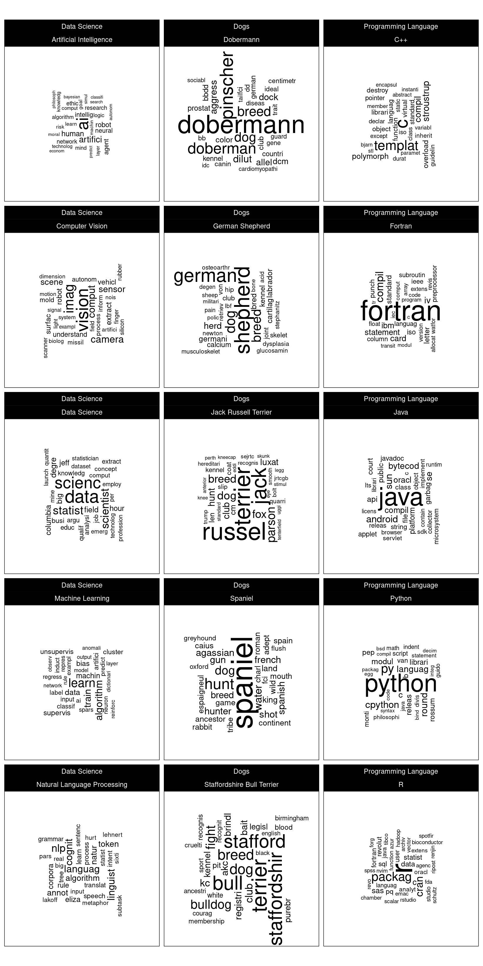
Figure 2.1: Word clouds faceted by document categories.
It is also insightful to remove the title words and recalculate the \(\mathrm{TFIDF}\) word cloud. The title words tend to overwhelm the other distinctive i.e. information-carrying words. The resulting word cloud is shown in figure 2.2.
# Utility function to remove stemmed title words.
eliminate_words <- function(title) {
    stringr::str_split(title, " ")[[1]] %>%
        tm::stemDocument() %>%
        stringr::str_to_lower()
}

df_tf_idf_no_tw <- df_tokens %>%
    dplyr::group_by(doc_id) %>%
    # Eliminate title words.
    dplyr::filter(!(word %in% eliminate_words(doc_id))) %>%
    # Remove acronyms and misspellings.
    dplyr::filter(!(doc_id == 'C++' & word == 'c')) %>%
    dplyr::filter(!(doc_id == 'Dobermann' & word == 'doberman')) %>%
    dplyr::filter(
        !(doc_id == 'Staffordshire Bull Terrier' & word == 'stafford')) %>%
    dplyr::filter(!(doc_id == 'Artificial Intelligence' & word == 'ai')) %>%
    dplyr::ungroup() %>%
    # Compute TFIDF
    dplyr::group_by(doc_class, doc_id) %>%
    dplyr::count(word, sort = TRUE) %>%
    dplyr::ungroup() %>%
    tidytext::bind_tf_idf(word, doc_id, n)

# Plot word cloud
plot_word_cloud(df_tf_idf_no_tw, max_size = 10)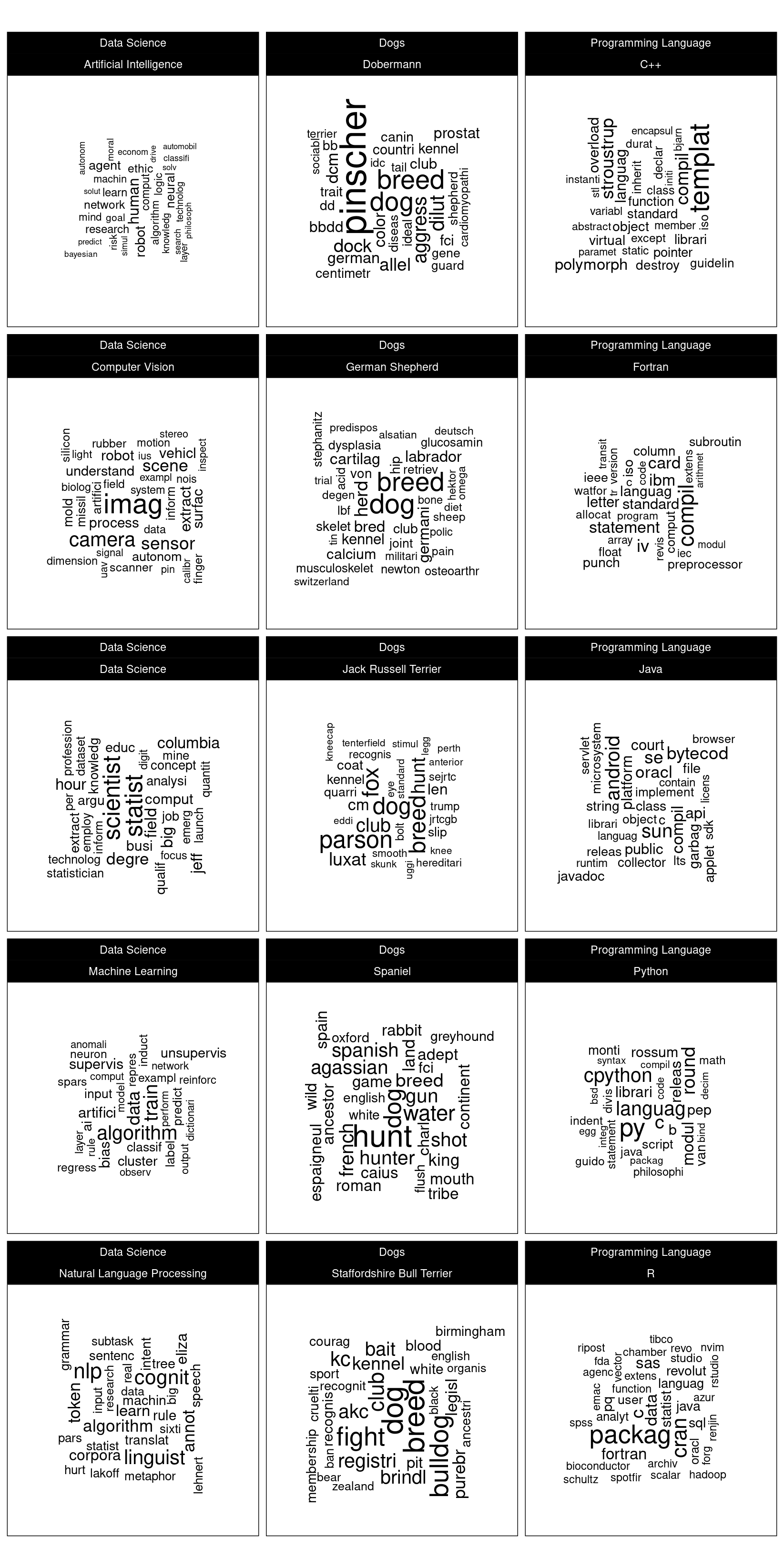
Figure 2.2: Word clouds faceted by document categories with title document title words removed from the corpus.
From figure 2.2 the high scoring words seem consistent with experience in these subjects and this confirms that the \(\mathrm{TFIDF}\) metric is a useful indicator of the words that best describe what is distinctive about the contents of a document.
Notice that the word ‘dog’ is significant for each of the 5 pages relating to dogs. This is to be expected since the word ‘dog’ is not a generally significant word for the 15 document corpus but is significant for these 5 articles. Therefore, the \(\mathrm{TFIDF}\) is relatively large. To demonstrate the usefulness of the \(\textrm{TFIDF}\) metric, it will be recalculated for only the dog articles. The resulting word cloud is shown in figure @ref{fig:plt-wordcloud-dogs}. It is observed that the word ‘dog’ is eliminated since although the absolute count of the word for each document has not changed, it is now common to all documents, hence the \(\mathrm{IDF}\) is 0.
df_tf_idf_dogs <- df_tokens %>%
    dplyr::filter(doc_class == 'Dogs') %>%
    dplyr::group_by(doc_class, doc_id) %>%
    dplyr::count(word, sort = TRUE) %>%
    dplyr::filter(!(word %in% eliminate_words(doc_id))) %>%
    dplyr::filter(!(doc_id == 'Dobermann' & word == 'doberman')) %>%
    dplyr::filter(
        !(doc_id == 'Staffordshire Bull Terrier' & word == 'stafford')) %>%
    dplyr::ungroup() %>%
    tidytext::bind_tf_idf(word, doc_id, n)

plot_word_cloud(df_tf_idf_dogs, max_size = 10)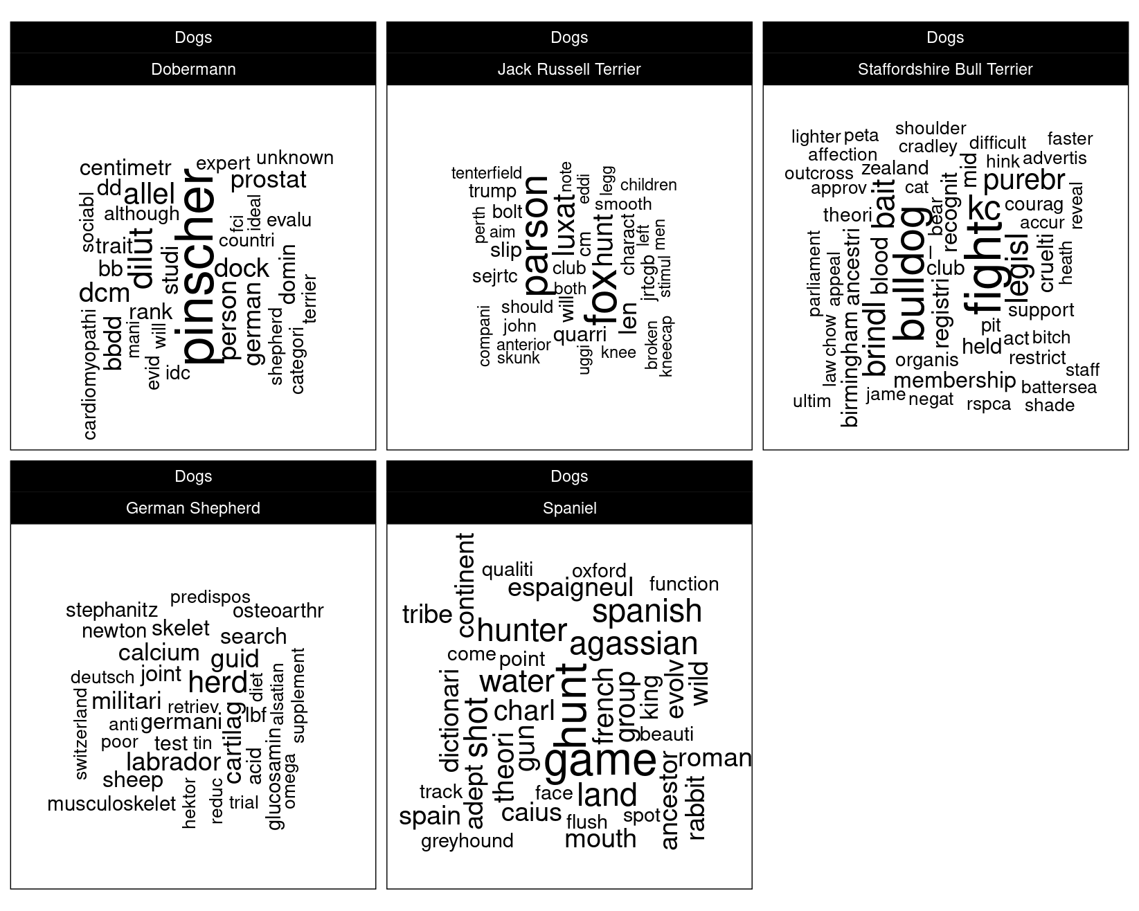
Figure 2.3: Word clouds for documents relating to dogs.
References
Feinerer, Ingo, and Kurt Hornik. 2019. Tm: Text Mining Package. https://CRAN.R-project.org/package=tm.
Robinson, David, and Julia Silge. 2020. Tidytext: Text Mining Using ’Dplyr’, ’Ggplot2’, and Other Tidy Tools. https://CRAN.R-project.org/package=tidytext.
Silge, Julia, and David Robinson. 2016. “Tidytext: Text Mining and Analysis Using Tidy Data Principles in R.” JOSS 1 (3). https://doi.org/10.21105/joss.00037.
Wickham, Hadley. 2019a. Rvest: Easily Harvest (Scrape) Web Pages. https://CRAN.R-project.org/package=rvest.
Wickham, Hadley, Jim Hester, and Jeroen Ooms. 2020. Xml2: Parse Xml. https://CRAN.R-project.org/package=xml2.